The q-Gaussian family

Visualize the q-Gaussian density across the entropic index and check that qjax.sample matches the analytic PDF.

What it shows

The q-Gaussian is the maximum-Tsallis-entropy distribution under a fixed second moment — the q-deformed analogue of the normal distribution. Written with the deformed exponential \(\exp_q(u) = [1 + (1-q)\,u]_+^{1/(1-q)}\), its density is

\[ \mathcal{G}_q(x) = \frac{\sqrt{\beta}}{C_q}\,\exp_q(-\beta x^2), \]

where \(\beta > 0\) sets the width and \(C_q\) is the normalizing constant.

The single index q controls the tails. For \(q < 1\) the support is compact — the density is exactly zero beyond a finite range. At \(q = 1\) it reduces to the ordinary Gaussian \(\sqrt{\beta/\pi}\,e^{-\beta x^2}\). For \(1 < q < 3\) it develops heavy, power-law tails: it is a rescaled Student-\(t\) with \(\nu = (3-q)/(q-1)\) degrees of freedom, whose variance is finite only for \(q < 5/3\).

The example plots this density family for \(q \in \{0.5, 1, 1.5, 2, 2.5\}\) and, on a second panel, overlays histograms of sampled draws on the analytic density to confirm the two agree.

How it works

The density and the sampler are one call each; beta sets the width.

import jax, jax.numpy as jnp
import qjax

x = jnp.linspace(-6.0, 6.0, 400)

# the density family across q (q = 1 is the standard Gaussian)
for q in (0.5, 1.0, 1.5, 2.0, 2.5):
    pdf = qjax.q_gaussian_pdf(x, q=q, beta=1.0)

# draw samples for 1 <= q < 3 and compare to the analytic density
samples = qjax.sample(jax.random.PRNGKey(0), q=1.5, beta=1.0, shape=(50_000,))

qjax.plots.plot_q_gaussian is a convenience helper that draws the left panel directly.

Result

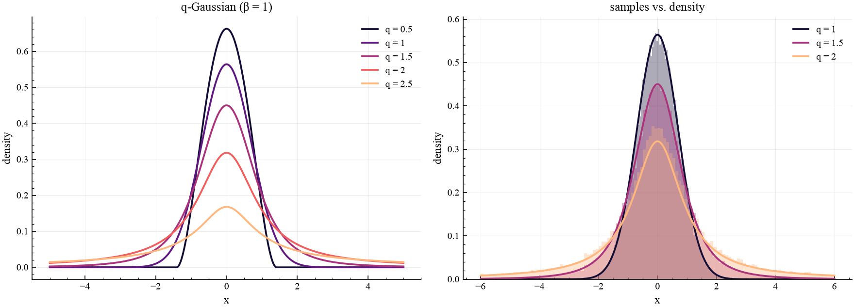
Left: the q-Gaussian density for several values of q (heavier tails as q grows). Right: sampled histograms (q = 1, 1.5, 2) overlaid on the analytic density — they match.

Takeaways

A single parameter q interpolates continuously from compact-support through the Gaussian to heavy-tailed distributions, so one family spans qualitatively different regimes. The closed-form density q_gaussian_pdf() and the sampler sample() are mutually consistent — the empirical histograms track the analytic curve. This same distribution underpins the maximum-likelihood example, where q itself is recovered from data.