Node classification under label noise

The same graph neural network, trained with a learnable Tsallis q, stays robust as training labels are corrupted — while the Shannon baseline (q = 1) propagates the noise across the graph.

What it shows

A two-layer graph convolutional network (GCN) is trained on a synthetic graph — a stochastic block model whose communities are the classes — while a growing fraction \(\eta\) of the training labels is corrupted at random. The only knob is the entropic index q of the tsallis_cross_entropy() loss,

\[ H_q(y, p) = -\sum_i y_i \ln_q p_i \;\xrightarrow{q \to 1}\; -\sum_i y_i \log p_i . \]

At \(q = 1\) this is exactly the Shannon baseline: the per-node loss \(-\log p_c\) is unbounded, so a confidently mislabeled node produces an enormous gradient — and because a GCN smooths predictions over edges, that error spreads to its neighbors. Making q learnable (training it jointly with the network) gives a bounded loss whose gradient saturates on hard or mislabeled nodes, so q descends into the robust regime on its own and clean-set accuracy degrades far more gracefully.

The task is transductive: a single graph, with a held-out set of test nodes whose labels stay clean. Every configuration is averaged over seeds.

How it works

The GCN propagates features over the symmetric-normalized adjacency \(\hat A = D^{-1/2}(A + I)D^{-1/2}\), and the loss is tsallis_cross_entropy on the softmax outputs, masked to the (noisy) training nodes:

import jax, jax.numpy as jnp
import qjax

def gcn_logits(params, x, a_hat):
    h = jax.nn.relu(a_hat @ (x @ params["w1"]))
    return a_hat @ (h @ params["w2"])

def loss_fn(params, x, a_hat, y_onehot, train_mask):
    # learnable q in (0.3, 1.3): spans the robust (q<1) and Shannon (q=1) regimes
    q = 0.3 + 1.0 * jax.nn.sigmoid(params["q_raw"])
    p = jnp.clip(jax.nn.softmax(gcn_logits(params, x, a_hat), axis=-1), 1e-7, 1.0)
    ce = qjax.tsallis_cross_entropy(p, y_onehot, q=q, axis=-1)
    w = train_mask.astype(jnp.float32)
    return jnp.sum(ce * w) / jnp.sum(w)  # mean over training nodes only

Set a fixed q = 1 instead of the learnable one to recover the Shannon baseline. Both share the same graph, initialization, noisy labels and optimizer — only q differs.

Result

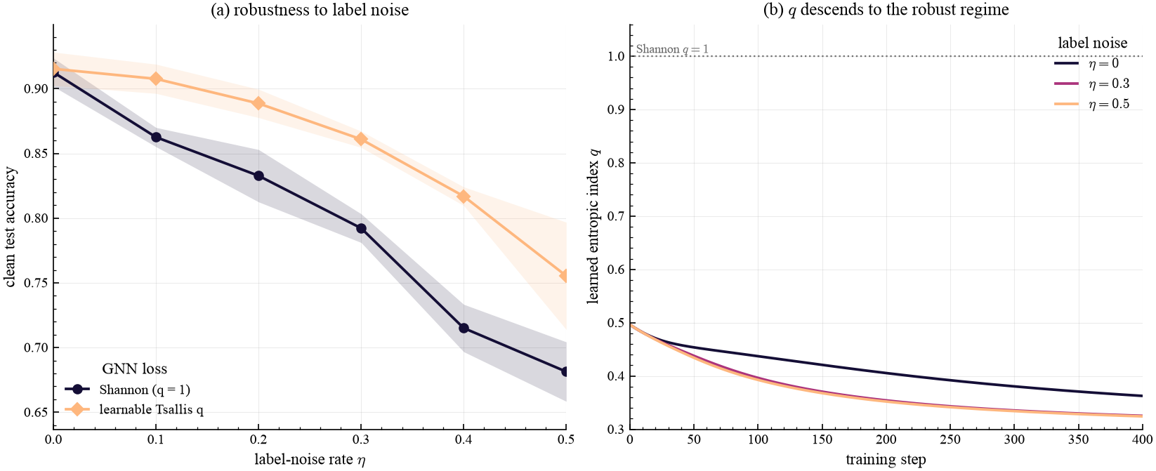
(a) Clean-test accuracy vs. label-noise rate η: the learnable-Tsallis GNN degrades far more gracefully than the Shannon baseline as noise grows. (b) The learnable q descends from its initialization into the robust regime (q < 1) during training, at every noise level.

The robustness is also visible on the graph itself. The same graph is shown at 40% label noise, nodes colored by each GNN’s prediction and misclassified test nodes ringed in red — the Shannon GNN is peppered with errors, while the learnable-Tsallis GNN stays visibly cleaner.

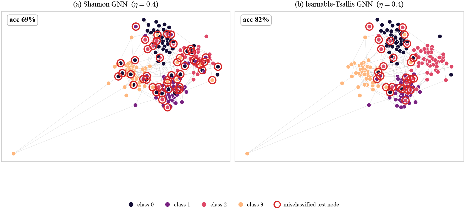
The same graph at η = 0.4, colored by each GNN’s prediction. (a) The Shannon baseline scatters wrong-class nodes across the communities; (b) the learnable-Tsallis GNN keeps the communities clean.

Takeaways

On graphs, where label noise is amplified by message passing, a learnable q again discovers a bounded, noise-robust loss with no grid search — mirroring the label-noise classification, attention and reinforcement learning results: the right amount of non-extensivity is found by gradient descent rather than by hand.